CX Matrix Decompositions for Tumour Classifications

In this example, we are going to replicate one of the experiements from the paper CUR matrix decompositions for improved data analysis, which uses data from Nielson et. al. (2002). We have a dataset of gene expressions for 3,935 genes from 31 different tumours, with three different cancer subtypes represented in the dataset, and the question we want to answer is: can we determine the type of tumour from just a handful of the 4,000 different genes?

We are going to do this by picking genes that have high leverage scores.

First step is to import the data:

import pandas
from spalor.models import CUR
from spalor.datasets import Nielsen2002
gex=Nielsen2002()
gex.head()

	GIST	GIST	GIST	GIST	GIST	GIST	GIST	GIST	GIST	GIST	...	LEIO	SARC	SARC	SARC	SARC	SARC	SARC	SARC	SARC	SARC
Gene
TACSTD2	-1.3650	-0.7588	0.33435	1.7160	0.18766	0.1467	0.3831	0.8449	-0.7469	0.9075	...	-0.2423	-1.9880	1.6110	-0.9822	-2.3360	-0.7156	-0.6364	1.8910	-0.4032	-0.3697
GJB2	-0.0950	0.3063	0.63040	0.7806	0.81530	-0.9518	-0.7240	-1.0940	-0.4872	-0.6808	...	-1.5760	0.0433	0.4723	-1.2890	-1.7290	-0.9109	-0.6991	-0.5254	-0.1763	-0.1103
CUGBP2	-0.6385	-0.2870	-0.17250	-0.5951	0.17030	0.6095	-0.1460	0.4343	-0.8280	-0.3281	...	0.1620	-0.0807	0.2439	-3.5830	-0.0795	0.8805	1.6600	2.0190	-0.2785	-0.2276
KIAA0080	-0.5501	1.0980	1.11400	1.0330	-0.34850	0.0632	-0.7378	0.0826	0.6216	-1.3870	...	0.9759	1.2240	-0.6170	-3.1070	0.6073	0.7063	-1.1070	0.5016	-0.0544	-0.7320
CED-6	-0.4295	-3.2950	-2.00600	0.5949	0.48850	-1.3600	-0.5136	-1.5670	1.5310	0.1229	...	-0.8084	0.2960	-0.8529	-1.9260	-0.5620	0.6970	0.8229	2.1340	2.0010	1.5360

5 rows × 31 columns

genes=gex.index.to_numpy();
cancer_type=gex.columns
data=gex.to_numpy().T

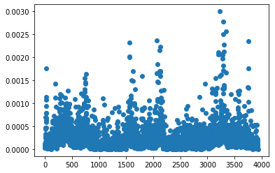
Theres a function in SpaLor for calculating the leverage scores. It requires a rank, but this is not the same as the number of columns we hope to sample. The leverage scores are how important a given column is when we are constructing a rank r approximation of the matrix. We are going to calculate and plot them here:

from spalor.matrix_tools import leverage_score
from matplotlib import pyplot as plt

ls=leverage_score(data,k=3, axis=1)
plt.plot(ls,'o')
plt.show()

A good way to think about this plot is that the genes in this plot that have a much larger leverage score than average are the ones that contain the most information. When we fit our data to a CX model from SpaLoR, its going to randomly sample genes with a probability proportional to the leverage score squared.

# from spalor.models.cx import CX
import numpy as np
import pandas as pd
cx=CX(n_components=30, method="exact")
C=cx.fit_transform(data)
C=pd.DataFrame(C, columns=genes[cx.cols], index=cancer_type)
print("genes selected: ",genes[cx.cols])

genes selected:  ['ANXA1' 'IGKC' 'FLJ20898' 'CSF2RB' 'RNF24' 'IGKC' 'C20ORF1' 'ZFHX1B'
 'RPS27' 'CD24' 'PCOLCE' 'DUSP6' 'EPS8' 'SSBP2' 'CEP2' 'GFRA2' 'FLJ20701'
 'KIAA0008' 'KIAA0300' 'FLJ14054' 'COPEB' 'IGF2' 'TYROBP' 'IMPA2' 'RAB39'
 'OSF-2' 'APLP2' nan 'EIF2B3' 'EDN3']

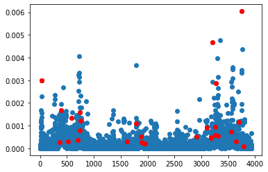
Here is the same plot as before with the selected genes highlighted red. Most of them have a high leverage score, but some do not.

plt.plot(ls,'o')
ls=leverage_score(data,k=1, axis=1)

#cols=np.where(20* ls > np.random.rand(*ls.shape))[0]
plt.plot(cx.cols, ls[cx.cols],'or')
plt.show()

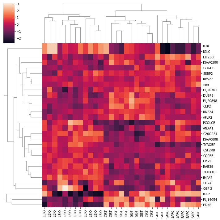
A clustermap of the genes shows the limited gene set can seperate the three different types of cancer.

import seaborn as sns
sns.clustermap(C.T, col_cluster=1, z_score=1)

<seaborn.matrix.ClusterGrid at 0x7f851d9ea370>